When designing a surveying network, it is important to know the accuracy of your observations in order to get a realistic estimate of the accuracy that can be achieved for the coordinates. For traditional observations such as total stations angles and distances, we usually rely on manufacturer specifications and experience. For GNSS baselines, this is more difficult, as the accuracy depends on factors such as the measurement duration and baseline length, where the latter may vary greatly.
I was tasked to compute a realistic estimate for GNSS baseline standard deviations, based upon a past measurement campaign that used 20-minute static GNSS surveys and baseline lengths between 3 meters and 90 kilometers. I had the individual standard deviations that were used and tested in the network adjustment, for some 8900 baselines.
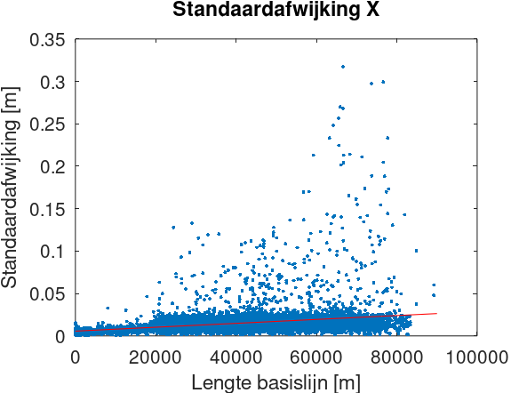
The simple approach would be to compute the mean or median standard deviation for each of the three baseline vector components. But since the accuracy is dependent on the baseline length, this would yield an optimistic accuracy for long baselines and a pessimistic accuracy for short baselines. Instead, we want to compute the constant and distance-dependent part of the standard deviation, which we will do via least-squares adjustment. The functional model is
s = a + b d
with s being the standard deviation as used in/reported by the network adjustment, a the constant part, b the distance-dependent part, and d the baseline length. This is linear, so we don’t need to iterate. The design matrix elements for each observation are obtained by linearization, each line of the design matrix containing
[1 d]
In my opinion, the easiest way to do the computation is in Octave. I did some preprocessing of the data in Excel (such as computing the baseline length from the baseline vector components), and created a text file with four columns: baseline length and the standard deviation of the X, Y, and Z components:
77733.06768	0.1443225	0.3188318	0.1335789

77754.58419	0.2333499	0.227157	0.178969

77755.33892	0.0163548	0.0061838	0.0186347

...
This file can be read in Octave this way:
fid=fopen("stdafw.txt","r");

[data,n]=fscanf(fid,"%f\n",[4,Inf]);

fclose(fid);
n is the number of elements read, so we need to divide it by 4 to get the number of observations and dimension the matrices that we need. We can then construct the design matrix and fill the observation vectors.
n=n/4;

A=zeros(n,2);

yx=zeros(n,1);

yy=zeros(n,1);

yz=zeros(n,1);
for i=1:n

A(i,1)=1;

A(i,2)=data(1,i)/1000;

yx(i,1)=data(2,i);

yy(i,1)=data(3,i);

yz(i,1)=data(4,i);

end
Computing the result is super easy in Octave:
xx=inv(A'*A)*A'*yx

xy=inv(A'*A)*A'*yy

xz=inv(A'*A)*A'*yz
We can then plot both the observations and the resulting fit (shown here only for X):
figure(1);

plot(data(1,:),yx,'.');

hold on;

x=[0;90000];

y=[xx(1);xx(1)+xx(2)*x(2)/1000];

plot(x,y,'-r');

xlabel("Lengte basislijn [m]");

ylabel("Standaardafwijking [m]");

title("Standaardafwijking X");